Subroutines when Computing Isogenies from Ideals
At a high level, the purpose of the algorithm IdealToIsogenyFromKLPT() is to compute the isogeny corresponding to a given ideal (via the Deuring Correspondence). We discuss how it is implemented in more depth in Computing Isogenies From Ideals.
In this blogpost, however, we discuss the two main subroutines in IdealToIsogenyFromKLPT():
IdealToIsogenyCoprime()to translate and evaluate $T$-isogenies (where $T$ is coprime to $\ell$)IdealToIsogenySmallFromKLPT()to translate $\ell^f$-isogenies using the output ofIdealToIsogenyCoprime().
Corresponding isogeny of ideal with coprime norm
We first describe IdealToIsogenyCoprime(), which takes as input two equivalent left $\OO_0$-ideals $J, K$ where $J$ has norm dividing $T^2$ and $K$ has $\ell$-power norm, as well as the connecting isogeny corresponding to $K$, namely $\varphi_K: E_0 \rightarrow E_K$. The output is the isogeny $\varphi_J : E_0 \to E_J$ corresponding to $J$.
As the two ideals are equivalent, we expect the domains and codomains of $\phi_I$ and $\phi_J$ to be isomorphic. The importance of this function is to find isogenies with coprime degrees which is important for various pushforwards and pullbacks in the parent algorithms which call IdealToIsogenyCoprime().
The algorithm can be broken down into the following steps:
Consider the function: $$\chi_I = I \frac{\bar{\alpha}}{n(I)}, \quad \alpha \in I \mathrel{\backslash} \{0\},$$ as defined in Lemma 1 in the SQISign paper. For the first step, we need to find $\alpha$ such that $\chi_K(\alpha) = J$, which is achieved using the function
chi_inverse().We compute two ideals $$H_1 = J + \OO_0T, \text{ and } \ H_2 = \OO_0\alpha + \OO_0\frac{n(J)}{n(H_1)}.$$ Ensure that the ideals are cyclic and that their norm divides $T$.
Compute the isogenies whose kernels correspond to the $H_i$, say $\varphi_i: E_0 \rightarrow E_i = E_0/\langle H_i \rangle$.
Compute an isogeny $$\psi : E_K\rightarrow E_{\psi} = E_K/\langle \varphi_K(\ker (\varphi_2)) \rangle ,$$ i.e., $\psi = [\phi_K]_\star \phi_2$ is the pushforward of $\varphi_2$ through $\varphi_K$. The codomain of $E_{\psi}$ should be isomorphic to $E_1$, but may not be equal. To fix this we use techniques described in Correct up to Isomorphism.
Compute the dual isogeny $\widehat{\psi}$. Throughout, we can ensure the computation of the dual isogenies is efficient by exploiting the fact we already know the kernel of $\psi$. For an isogeny of degree $D$, we find $\ker(\widehat{\psi}) = \psi(R)$ for some point $R \in E[D]$ linearly independent to $\ker(\psi)$. By the previous step, the codomain of $\varphi_1$ and the domain of $\widehat{\psi}$ should be the same.
Return $$\varphi_J = \widehat{\psi} \circ \varphi_1: E_0 \rightarrow E_1 \rightarrow E_K \cong E_J = E_0/\langle J \rangle.$$
Corresponding isogeny of ideal with norm $\ell^{2f_{\text{step}} + \Delta}$
Next, we describe the subroutine IdealToIsogenySmallFromKLPT() in more detail. This algorithm takes the following input: left $\OO_0$-ideals $I$ and $J$ of norm dividing $T^2\ell^{2f_{\text{step}}+\Delta}$ and $T^2$ (respectively), an ideal $K \sim J$ of $\ell$-power norm, and the isogenies $\varphi_J$, $\varphi_K$ from $E_0$ to $E_1$ corresponding to $J$, $K$ respectively. It will output:
- $\varphi: E_1 \rightarrow E_2$ of degree $\ell^{2f_{\text{step}}+\Delta}$, such that $\varphi_I = \varphi \circ \varphi_J$,
- $L \sim I$ of norm dividing $T^2$
- The corresponding isogeny $\varphi_L : E_0 \to E_2$.
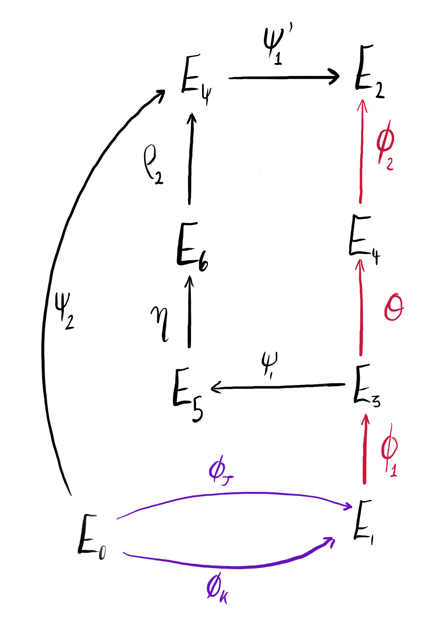
Figure 1: We compute $\varphi$ using the isogeny diagram above. The isogenies in purple are given as input, and those in red are computed within the algorithm to obtain $\varphi$.
Following the diagram above, we compute $\varphi: E_1 \rightarrow E_2$ and $\varphi_L : E_0 \to E_2$ as:
- $\varphi = \psi_1^\prime \circ \rho_2 \circ \eta \circ \psi_1 \circ \varphi_1$.
- $\varphi_L = \psi_1’ \circ \psi_2$
We will do this as follows:
Compute $\varphi_1: E_1 \rightarrow E_3$: we first compute the kernel corresponding to $I_1 = I + \OO_0\ell^{\text{step}}$ of norm dividing $\ell^{\text{step}}$. Let $P$ be the generator of this kernel. As $I_1$ is a left $\OO_0$-ideal, $P \in E_0$. As $\varphi_1$ has domain $E_1$, we map $P$ to $E_1$ using $\varphi_J: E_0 \rightarrow E_1$. Then, $\varphi_1: E_1 \rightarrow E_1/\langle \varphi_J(P) \rangle.$
Compute ideal $L$: we now use KLPT to compute the ideal $L$ equivalent to $I$ with norm dividing $T^2$ by running
EquivalentSmoothIdealHeuristic().Compute $\gamma$: we compute $\alpha$ such that $\chi_K(\alpha) = J$, and $\beta$ such that $\chi_I(\beta) = L$ using
chi_inverse(). Set $$\gamma = \frac{\beta\alpha}{n(J)}.$$ Be careful: when $n(K) = 1$,chi_inverse()will return $\pm i$. This means that when we compute kernels from $\gamma$, it may be twisted by the automorphism $\iota$. To avoid this, we manually set $\alpha = 1$.Compute $\psi_1$: as the domain of $\psi_1$ is not $E_0$, we need to instead consider a related ideal with left order $\OO_0$. The ideal we consider is $$H_1 = \OO_0\gamma + \OO_0(n(K)\ell^{f_{\text{step}}}T),$$ which will correspond to the isogeny $$\phi_{H_1} = \psi_1 \circ \varphi_1 \circ \varphi_K: E_0 \rightarrow E_5$$ of degree $n(K)l^{f_{\text{step}}}T$. Note that the $\ell$-power part of $H_1$ corresponds entirely to $\varphi_1 \circ \varphi_K$ as $\deg (\varphi_1) = \ell^{f_{\text{step}}}$ and $\deg (\varphi_K) = n(K)$. Therefore, we only need to compute the part of $H_1$ coprime to $\ell$, namely $H^\prime_{1} = \OO_0\gamma + \OO_0T$. From this, which we obtain $\psi_1$ by running
ideal_to_kernel()on $H^\prime_1$ to obtain kernel generator $P$. As $H^\prime_1$ has left order $\OO_0$, $P \in E_0$. Therefore, the kernel of $\psi_1$ is generated by $\varphi_1(\varphi_K(P)) \in E_3$.Compute $\psi_2$ and $\widehat{\rho}_2$: we now consider the ideal $$H_2 = \OO_0\bar{\gamma} + \OO_0\frac{n(\gamma)}{n(H_1)}\ell^{-\Delta}.$$ Then, $H_2$ has left order $\OO_0$ and will correspond to the isogeny $\varphi_{H_2} : E_0 \rightarrow E_6$ of degree dividing $\ell^{f_{\text{step}}}T$. How can this be used to compute $\psi_2$ and $\widehat{\rho}_2$?
- This isogeny can be decomposed as $\widehat{\rho}_2 \circ \psi_2: E_0 \rightarrow E_{\psi} \rightarrow E_6$ where $\widehat{\rho}_2$ is of degree dividing $\ell^{f_{\text{step}}}$ and $\psi_2$ is of degree dividing $T$.
- Compute $\ker(\varphi_{H_2})$ by running
ideal_to_kernel()on $H_2$. - Then, $\ker(\psi_2)$ is the subgroup of order (dividing) $T$ within $\ker(\varphi_{H_2})$, i.e., $\ker(\psi_2) = l^h\cdot \ker(\varphi_{H_2}),$ where $h$ is the $\ell$-valuation of $n(H_2)$. From this kernel we obtain $\psi_2: E_0 \rightarrow E_{\psi}$.
- Similarly, we compute the subgroup of $\ker(\varphi_{H_2})$ of order $\ell^{f_{\text{step}}}$ and push it through $\psi_2$ to obtain $\ker(\widehat{\rho}_2)$, and therefore $\widehat{\rho}_2$.
Meet-in-the-middle step to find $\eta$: we now brute force the isogeny $\eta: E_5 \rightarrow E_6$ of (small) degree $\Delta$ by using meet-in-the-middle. For more details on this, see the page Meet in the Middle Isogenies.
Recall that the desired output of this function is: $\varphi: E_1 \rightarrow E_2$ such that $\varphi_I= \varphi \circ \varphi_J$, an ideal $L \sim I$ and the corresponding isogeny $\varphi_L$. We now have all the pieces we need, but to output everything correctly, we will need to perform some pushforwards and pullbacks.
To compute $\varphi$, we exploit the fact that we know $\varphi_1 : E_1 \rightarrow E_3$, and $\varphi = \varphi_2 \circ \theta \circ \varphi_1$. For the other outputs, we have already computed $L$ in Step 2, and the corresponding isogeny is given by $\psi_1^\prime \circ \psi_2: E_0 \rightarrow E_2$, for which we computed $\psi_2$ in Step 5. We are left to compute $\psi_1^\prime$ and $\varphi_2 \circ \theta$.
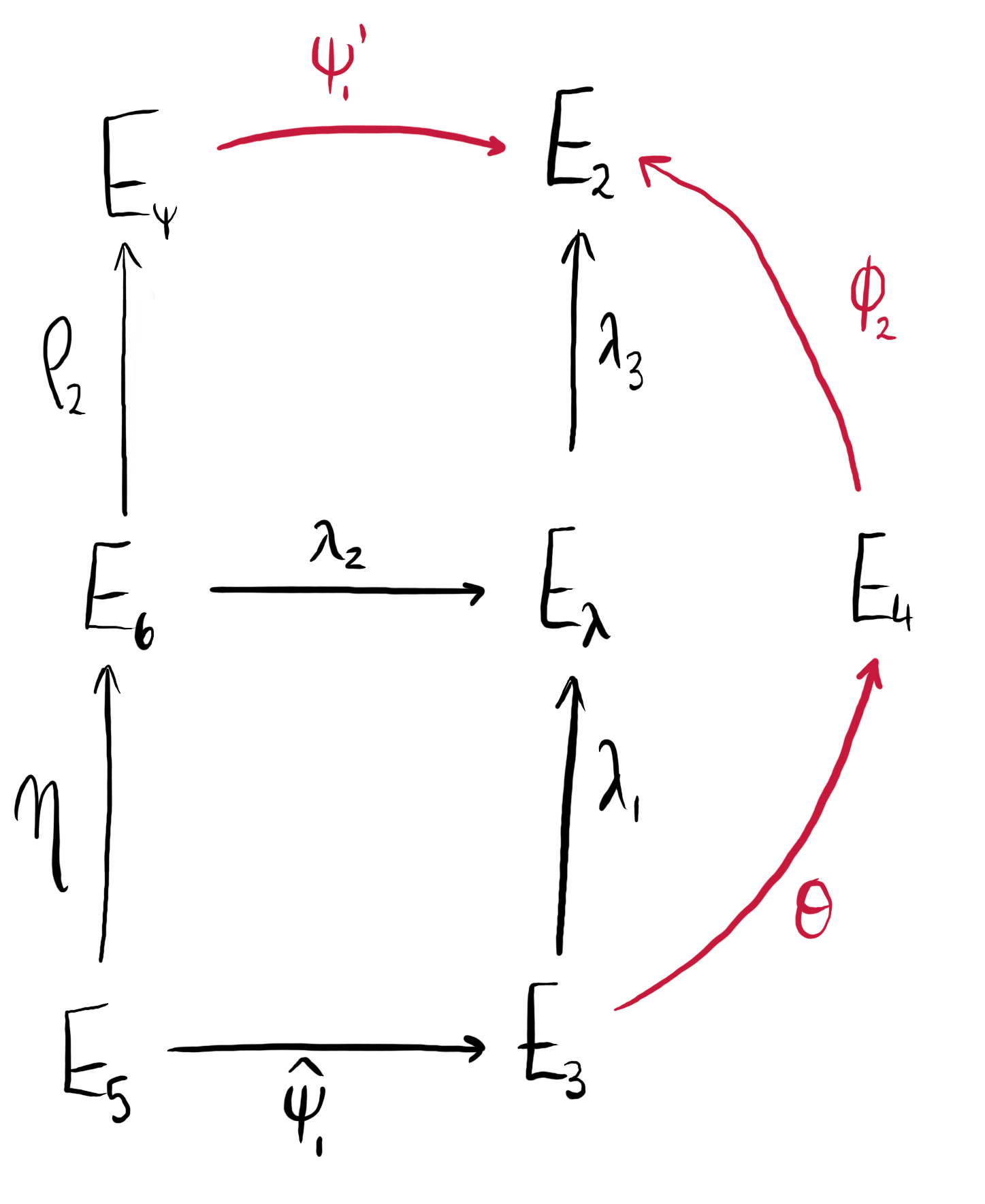
Figure 2: We compute $\psi_1^\prime$ and $\varphi_2 \circ \theta$ (shown in red) by considering the isogeny diagram above.
Compute $\psi_1^\prime$: from the diagram we can see that $$\ker(\psi_1^\prime) = \rho_2(\eta(\ker(\widehat{\psi}_1))),$$ so once we compute the dual of $\psi_1$, we can compute $\ker(\psi_1^\prime)$, and therefore $\psi_1^\prime$.
Compute $\varphi_2 \circ \theta$: ideally, we would compute the kernel of $\varphi_2 \circ \theta$ by observing that it is equal to $\widehat{\psi}_1(\ker(\rho_2 \circ \eta))$. However, we do not actually know the kernel of $\rho_2 \circ \eta$, so we work around this by computing $\lambda_1$ and $\lambda_3$ as $\varphi_2 \circ \theta = \lambda_3 \circ \lambda_1$. We do this, using the diagram above, as follows:
- We first compute $\ker(\lambda_1) = \widehat{\psi}_1(\ker(\eta))$ and from this we get $\lambda_1: E_3 \rightarrow E_{\lambda}$.
- To compute $\lambda_3$, we first need $\lambda_2$, whose kernel is given by $\eta(\ker(\widehat{\psi}_1))$. Then, by pre-composing with an isomorphism if necessary to make its codomain $E_{\lambda}$, we obtain $\lambda_2: E_6 \rightarrow E_{\lambda}$.
- Finally, we compute the kernel of $\lambda_3$ as $\lambda_2(\ker(\rho_2))$ to obtain the isogeny $\lambda_3: E_{\lambda} \rightarrow E_2$.
We can now output $\varphi$, $L$, and $\varphi_L$ as required.
Edge cases
Small step size
When the step size is small enough, i.e., smaller than $f_{\text{step}}$, we can avoid going through the entire procedure above as the isogeny we wish to compute has degree dividing the available torsion, and we can skip many of the tricks used above and simply directly compute the kernel from the ideal. Concretely, we simply do the following:
- Set $\varphi_J$ and $\varphi_K$ to have the same codomain as above.
- Derive $\varphi_1$ as above.
- Find $L$, an ideal equivalent to $I$ with norm dividing $T^2$.
We then return $\varphi_1$ and $L$. This will only happen when IdealToIsogenySmallFromKLPT() is called as the last step of the parent IdealToIsogenyFromKLPT().
Backtracking: when $\gamma$ has non-trivial GCD
There is a caveat with the procedure depicted above. Before computing $H_i$ in IdealToIsogenySmallFromKLPT() the coefficients of $\gamma$ (when written as a linear combination of the basis elements of $\OO_0$) may have non-trivial GCD, which causes the isogenies to backtrack and the algorithm to fail. One solution is to regenerate $L$ and $\gamma$ until the coefficients of $\gamma$ have trivial GCD. However, we can relax the condition by fixing this backtracking when the GCD is a power of $\ell$. We detail this procedure below.
Let $\alpha_1, \dots, \alpha_4$ be a basis of $\OO_0$, and write $\gamma = c_1\alpha_1 + \dots + c_4\alpha_4$. Let $g = \gcd(c_1, \dots, c_4)$. If $g \neq \ell^{\times}$, we regenerate $L$ and $\gamma$. Otherwise, let us say $g = \ell^d$. We replace $\gamma$ with $\gamma/g$. Note that now will have $g\cdot \gamma \in K$, $g\cdot\bar{\gamma} \in L$, and $$n(\gamma) = \frac{n(I)n(L)n(K)}{g^2n(J)}.$$ The ideals $H_1, H_2$ are computed in the same way, but in the meet-in-the-middle step we now expect to find an isogeny of degree $\ell^{\Delta + d}$ between $E_5$ and $E_6$.