Computing Isogenies from Ideals
Fundamental to SQISign is the Deuring correspondence. This gives us a link between the world of elliptic curves and the world of quaternion algebras over $\mathbb{Q}$. In particular, it tells us that the endomorphism ring of a supersingular elliptic curve $E$ defined over $\mathbb{F}_{p^2}$ is isomorphic to a maximal order in $\mathcal{B}_{p, \infty}$, the unique quaternion algebra ramified exactly at $p$ and $\infty$ (up to isomorphism). This correspondence extends to the maps between the elliptic curves: an isogeny $\phi: E \rightarrow E^\prime$ of degree $D$ between supersingular curves corresponds to a left integral $\mathcal{O}$-ideal $I$ of norm $D$, where $\text{End}(E) = \mathcal{O}$. $I$ is also a right $\mathcal{O}^\prime$-ideal, where $\text{End}(E^\prime) = \mathcal{O}^\prime$.
In this post, we will describe the algorithm IdealToIsogenyFromKLPT(), which computes the isogeny whose kernel corresponds to an input ideal $I$ with left order $\mathcal{O}$. The code which implements this is available at deuring.py, and is heavily commented.
Throughout, we will make reference to the special supersingular curve $E_0: y^2 = x^3 + x$ with known endomorphism ring $\text{End}(E_0) = \langle 1, \iota, \frac{\iota + \pi}{2}, \frac{1+\iota\pi}{2}\rangle$, where:
$$ \iota: (x,y) \mapsto (-x, \sqrt{-1}y), \qquad \pi: (x,y) \mapsto (x^p, y^p). $$
$\text{End}(E_0)$ isomorphic to the maximal order $\mathcal{O}_0 = \langle 1, i, \frac{i+j}{2}, \frac{1+ij}{2}\rangle$, where $i^2 = -1$ and $j^2 = -p$, via the isomorphism taking $\iota \mapsto i$ and $\pi \mapsto j$.
If our input ideal $I$ is a left $\mathcal{O}$-ideal with $\mathcal{O} \neq \mathcal{O}_0$, we actually need more information to compute the corresponding isogeny; we require the knowledge of a connecting ideal $K$ with left order $\mathcal{O}_0$ and right order $\mathcal{O}$, and its corresponding isogeny $\varphi_K: E_0 \rightarrow E$, where $\text{End}(E) \cong \mathcal{O}$. Indeed, to obtain the kernel corresponding to an ideal $I$, we need to know how to map elements of $I$ to endomorphisms of $E$. While we know that, abstractly, the endomorphism ring of $E$ is isomorphic to $\mathcal{O}$, we do not know an explicit (i.e. computable) isomorphism. As we shall see, we can effectively solve this by using a connecting isogeny $E_0 \rightarrow E$ of degree coprime to the norm of $I$.
On input of two ideal $I$, $K$, with norm $\ell^{\times}$, and corresponding isogeny $\varphi_K$ (as above), the algorithm IdealToIsogenyFromKLPT() proceeds as follows.
Step 1: Ideal filtration
We first compute a chain of ideals
$$ I = \tilde{I}_v \subset \dots \subset \tilde{I}_1 \subset \tilde{I}_0, $$
where each quotient $I_m = \tilde{I}_{m}/\tilde{I}_{m-1}$ has norm $\ell^{\text{step}}$, for some step size, and will correspond to an isogeny $\psi_m$. We will work with these quotients to break up the corresponding isogeny into smaller sized pieces, so that the kernel can be defined over $\mathbb{F}_{p^2}$. Otherwise, directly computing the isogeny corresponding to $I$ would require a large field extension over which to define the kernel points.
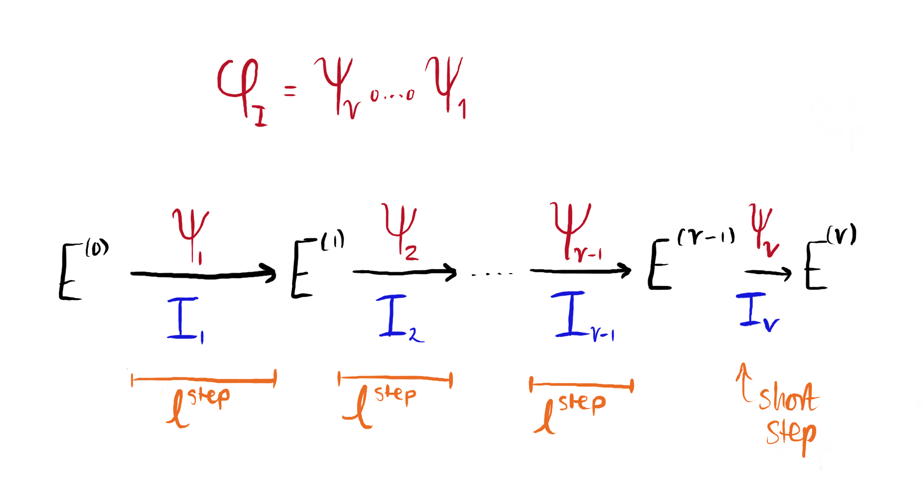
Figure 1: We break up $\varphi_I$ into small steps $\psi_m$ using ideal filtration on $I$.
By construction of the parameters, the largest power of $\ell$ dividing $p^2-1$ is $\ell^f$ (or equivalently, $f$ is the $\ell$-valuation of the order of a supersingular $E$ over $\mathbb{F}_{p^4}$). Therefore, a first choice for $\text{step}$ is $f$.
Following the SQISign paper, IdealToIsogenySmallFromKLPT() gives tricks to increase $\text{step}$ to $2f_{\text{step}}+\Delta$, where $f_{\text{step}}= f - \epsilon$, for some small positive integer $\epsilon$. We require that $\epsilon > 0$, as we need to be able to access the $2^{f_{\text{step}} + 1}$ torsion when performing endomorphism evaluations. See the page Between Kernels and Ideals for more context.
The integer $\Delta$ used to increase the step size corresponds to a brute force computation of an isogeny $\eta$ of degree $\ell^{\Delta}$. As this computation takes $O(\sqrt{\ell^{\Delta}})$ time, $\Delta$ cannot be too large. For details on how this brute force search is implemented see the page Meet in the Middle Isogenies.
If the norm of $I$ is not divisible by $2f_{\text{step}} + \Delta$, then the final quotient $I_\nu$ obtained from the filtration will only have norm $n(I_\nu) \mathrel{|} \ell^{2f_{\text{step}} + \Delta}$. Due to this, for the $m$-th step, we let $\Delta_\text{actual} = \max( n(I_m) - 2f_{\text{step}}, 0)$ (we do not want $\Delta_\text{actual}$ to be negative). If $\Delta_\text{actual} = 0$, we set $f_{\text{step}} = \frac{n(I_k)}{2}$. For clarity of presentation, we will drop the subscript and denote $\Delta_{\text{actual}}$ simply by $\Delta$.
Step 2: Find equivalent ideal with smooth norm
Using EquivalentSmoothIdealHeuristic(), we find an ideal $J$ that is equivalent to $K$ and is of smooth degree dividing $T^2$.
In some cases, we will already know an ideal of prime norm equivalent to $K$. In these cases, we can remove the call to the subroutine EquivalentPrimeIdealHeuristic(). This is particularly important for the case when $K$ is equivalent to an ideal with small norm (see the page Small Steps from Curves with Small Endomorphisms for more details).
Step 3: Compute the isogeny corresponding to $J$
The norm of $J$ (which divides $T^2$) is coprime to the norm of $K$ (which is $\ell^{\times}$), and so to compute the isogeny $\varphi_J$ corresponding to $J$, we use IdealToIsogenyCoprime(), which we describe in more detail in our blogpost Subroutines when Computing Isogenies from Ideals.
Step 4: Isogenies from filtration
We now compute the isogeny corresponding to each quotient. We skip the first ideal in the filtration $I_0$ as is the unit ideal of $\OO$.
For each ideal in the filtration, we want to compute the corresponding isogeny $\psi_m$.
Let $K_1 = K$ and $\varphi_{K_1} = \varphi_K$. For each step $m = 2, \dots, v$, we define
$$ \begin{aligned} K_m &= K \cdot I_{1} \cdot \dots \cdot I_{m-1} \\ \varphi_{K_m} &= \psi_{m-1} \circ \dots \circ \psi_1 \circ \varphi_K. \end{aligned} $$
After computing $\psi_m$, we update $K_{m-1}$ and $\varphi_{K_{m-1}}$ to obtain $K_m$ and $\varphi_{K_{m}}$, respectively.
To compute $\psi_m$ we first multiply ideals $J$ and $I_m$ to obtain $JI_m$. We do this because $JI_m$ has left ideal $\OO_0$ so the corresponding isogeny will be easier to compute, whereas in general, $I_m$ will not.
We compute the isogeny corresponding to $JI_m$, say $\varphi_{m}$, which satisfies $\varphi_m = \psi_m \circ \varphi_J$. As we know $\varphi_J$, we use this to find $\psi_m$. This procedure is done with IdealToIsogenySmallFromKLPT(). This is the most technical subroutine of the algorithm, as well as being the bottleneck step (primarily as it must be called for all ideals in the filtration). We describe it in more detail here in our blogpost Subroutines when Computing Isogenies from Ideals.
Before moving to the next step, there is one final detail to explain. To multiply the ideals $J$ and $I_m$ we need the left order of $J$ to match the right order of $I_m$ (not just isomorphic). However, this in general is not the case. We therefore have to supply our multiply_ideals() function with an automorphism that takes $I_m$ to an ideal with correct right order. For more information on this, see Correct up to Isomorphism.
Step 5: Patch together the isogeny factors
From the previous step, we get a list of isogeny factors that correspond to the ideals in the filtration. We now want to patch them together to obtain our desired isogeny $\varphi_I$. This can be done by composing the isogeny factors as $\psi_v \circ \dots \circ \psi_1$ using SageMath’s in-built funciton EllipticCurveHom_composite().
Recall that the Deuring correspondence is only true up to isomorphism, so we may have that the codomain of $\psi_m$ is not equal to the domain $\psi_{m+1}$, only isomorphic. Due to this, we may have to post-compose $\psi_{m+1}$ with such an isomorphism.
Edge cases
Small steps from $E_0$
We run IdealToIsogenyFromKLPT() in both keygen() and reponse() and for each of these cases we have to take some precautions with how the ideal filtration
is performed. The issue is, when we are working with an ideal $I$ which has particularly small norm, EquivalentPrimeIdealHeuristic() is likely to fail and
thus the KLPT algorithm cannot complete. This becomes a problem when we work with some ideal which via the Deuring correspondence is equivalent
to some isogeny $\phi : E_0 \to E$ of small degree.
Exactly how we deal with these edge cases takes some explaining, so we made a separate page called Small Steps from Curves with Small Endomorphisms, in which this is discussed in detail. The end claim is
that for IdealToIsogenyFromKLPT(), for keygen() to run successfully we must take the smallest step in the filtration chain first and for response() we must take the smallest step last.
This is controlled with the optional bool end_close_to_E0 available to IdealToIsogenyFromKLPT(). When end_close_to_E0 = True, we have the smallest step first and last otherwise.