Meet in the Middle Isogenies
During IdealToIsogenySmallFromKLPT(), two isogenies $\psi_1 : E_3 \to E_5$,
and $\psi_2 : E_\psi \to E_6$ are computed. The codomains of these isogenies
are separated by an unknown
degree $\ell^\Delta$ isogeny $\eta: E_5 \to E_6$. To compute the output
of the function IdealToIsogenySmallFromKLPT(), the isogeny $\eta$
must first be recovered through brute force.
The SQISign paper recommends implementing this as a meet in the middle
algorithm which will have complexity $O(\sqrt{\ell^{\Delta}})$.
This page details our implementation of this algorithm. Although the meet in
the middle search is not the bottleneck of IdealToIsogenySmallFromKLPT(),
we are interested in optimising this computation as it has utility outside of
the context of SQISign.
As implemented, we have assumed that both $\ell$, and $\Delta$ are small, so that we are unconcerned with memory management for the algorithm.
Overview
Assume we are given two curves $E_1$, $E_2$ which are connected by an unknown isogeny of known degree $\ell^\Delta$. The general idea of the meet in the middle algorithm is to enumerate all possible walks in the supersingular isogeny graph of length $\Delta/2$ starting from both $E_1$ and $E_2$. Then, we look at the intersection of the nodes at the end of each graph to discover the middle curve $E_m$. Given the graphs, it is efficient to compute the walk from $E_i$ to $E_m$. Concatenating these paths together gives the isogeny path from $E_1$ to $E_2$, and from this, we can compute the unknown isogeny.
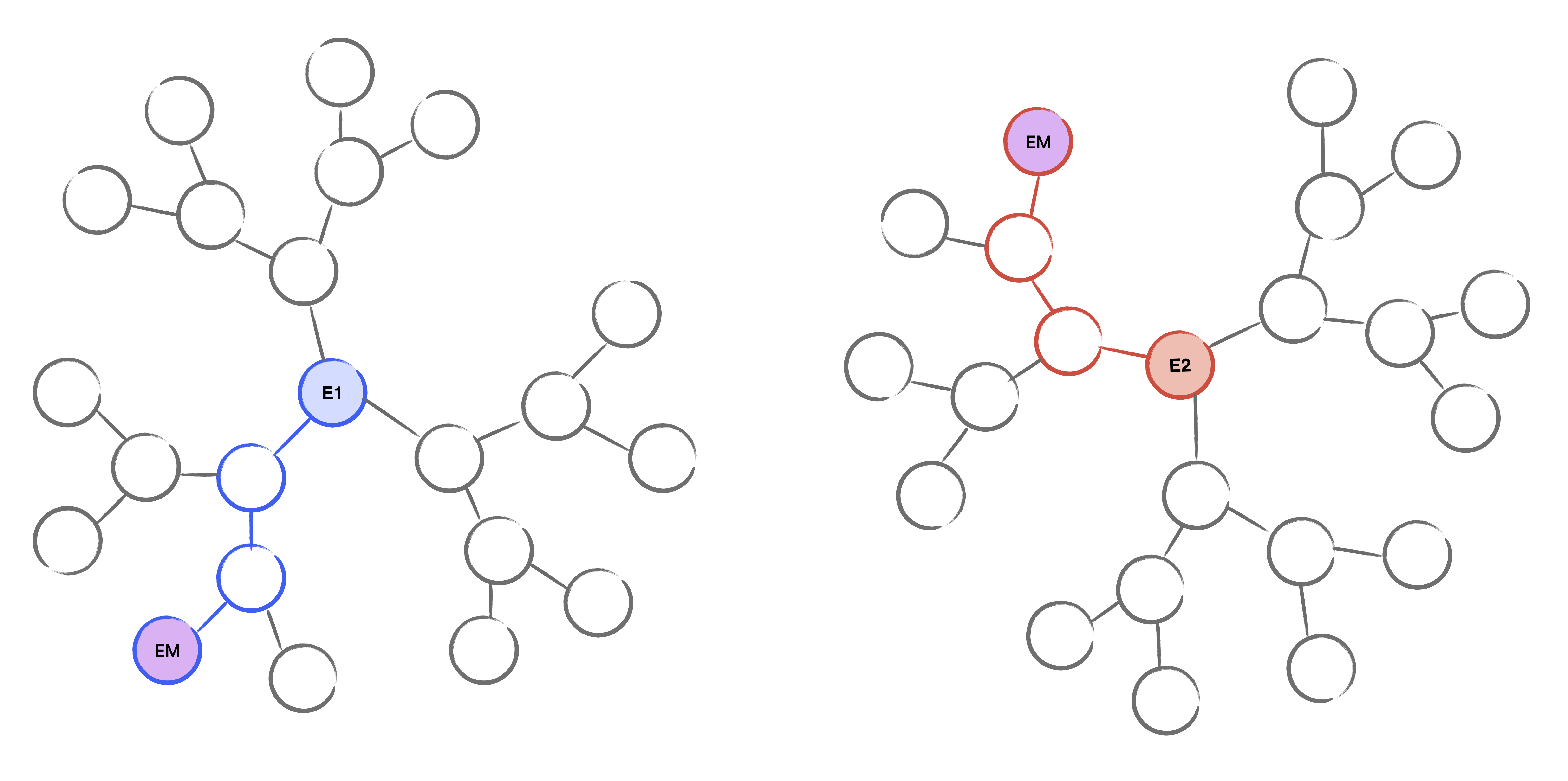
Figure 1: Supersingular isogeny graphs from both $E_1$ and $E_2$. The middle curve $E_m$ is found at level three for each graph.
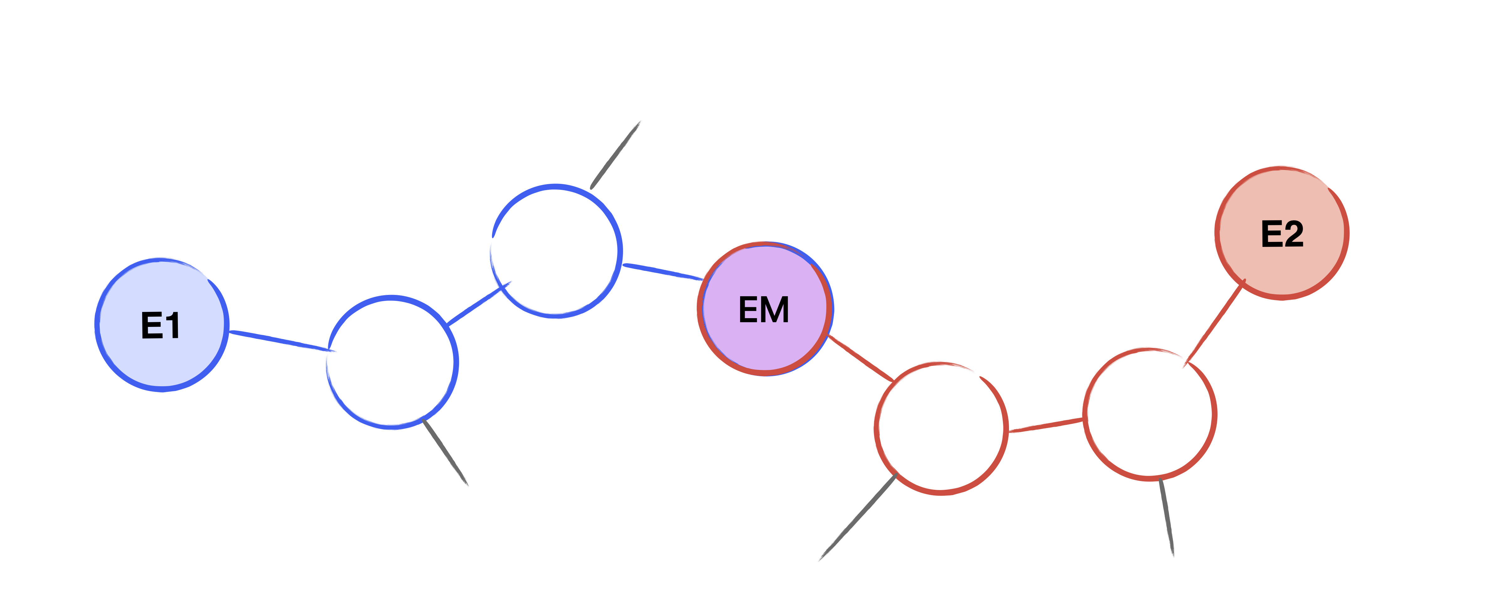
Figure 2: The derived path between $E_1$ and $E_2$ via the middle curve $E_m$, which was found in the meet in the middle search.
The algorithm can be broken down into the following steps:
- Compute a graph $G_1$ with $j$-invariants as nodes and $\ell$-isogenies as edges. The root of the graph will be $j_1 = j(E_1)$, from which we take walks of length $e_1 = \lfloor \Delta/2 \rfloor$ to obtain the middle $j$-invariants at level $e_1$.
- Compute a second graph $G_2$ with $j_2 = j(E_2)$ as the root and depth $e_2=\Delta-e_1$.
- Set $j_m$ to be the intersection $G_1[e_1] \cap G_2[e_2]$. If the intersection is empty, terminate the algorithm with an error that no isogeny can be found. Note that we can compute this intersection as we generate $G_2$ and terminate as soon as $j_m$ has been discovered.
- Compute a path $p_i$ from $j_i$ to $j_m$ for each graph $G_i$. Concatenate the paths to compute a path $p$ which walks from $j_1$ to $j_2$.
- For each step of the path, we now want to compute the corresponding $\ell$-isogeny. The path starts on node $j^{(1)} = j_1$, which corresponds to $E^{(1)} = E_1$. For each step in the path $p$, brute force all $\ell$-isogenies from $E^{(i)}$ until an isogeny is found from $\phi_i : E^{(i)} \to E^{(i+1)}$ with $j(E^{(i+1)}) = j^{(i+1)}$. Store $\phi_i$.
- Compose all $\ell$-isogenies $\phi_i$ to compute the $\ell^{\Delta}$-isogeny $\phi = \phi_\Delta \circ \ldots \circ \phi_1$.
- As this chain is derived from the $j$-invariants, we must ensure that the codomain of $\phi$ is $E_2$ by finally post-composing with the correct isomorphism.
The code which implements this is available at
mitm.py
and is commented throughout. The remainder of this page looks at some of the
implementation choices we made for each step outlined above.
Computing the isogeny graphs
As implemented, the data structure for the graph is crude. If someone reading this knows of something more efficient, we would love to hear from you.
Each level in the graph is a dictionary with nodes as keys and parent nodes as values. This structure was picked such that given a node at level $i$, we can efficiently find the parent node at level $(i-1)$ and work backwards towards the root. The graph itself is simply a list of the level dictionaries, with the root at the zero-index and middle values at the end.
The graph itself is built using a depth-first search. This has no bearing on the computation of $G_1$, for which we must compute the entire graph, but it means we compute as few nodes as possible for $G_2$ while searching for the middle j-invariant.
Computing neighbouring j-invariants
To compute the node values, the naïve method would be to compute all $\ell$-isogenies from the starting curve and then store the $j$-invariant of the codomain as the node data for each step. However, we can compute the neighbouring $j$-invariants without computing isogenies, by instead computing roots of a special polynomial: the modular polynomial.
The modular polynomial $\Phi_{\ell}(X,Y)$ has the special property that given $j_1 = j(E_1)$, the roots of $\Phi_{\ell}(j_1,Y) \in \mathbb{F}_{q}[Y]$ are the $j$-invariants of the elliptic curves which are connected to $E_1$ by a cyclic isogeny of degree $\ell$. This means that given a node with $j$-invariant $j^{(i)}$, we can compute the $j$-invariants of all neighbouring nodes as the roots of $\Phi_{\ell}(j^{(i)},Y)$.
As our elliptic curves are supersingular, all $j$-invariants of curves $\ell$-isogenous to $E^{(i)}$ will be elements of $\mathbb{F}_{p^2}$, which means we can work in $\mathbb{F}_{p^2}$ when computing roots, even if we are working with curves $E / \mathbb{F}_{p^{2k}}$.
For the case of SQISign, we have $\ell = 2$ and the modular polynomial is given by:
$$ \begin{aligned} \Phi_2(X,Y) &= X^3 - X^2Y^2 + 1488X^2Y - 162000X^2 + 1488XY^2 \\ &+ 40773375XY + 8748000000x + Y^3 - 162000Y^2 \\ &+ 8748000000Y - 157464000000000. \end{aligned} $$
For the first node in the graph, all we have is the j-invariant for the starting curve, and so we must find all roots of the modular polynomial above. We can do this relatively easily in SageMath, however it is not a fast computation. The code which implements this is below and should be straightforward.
def generic_modular_polynomial_roots(j1):
    """
    Compute the roots to the Modular polynomial
    Φ2, setting x to be the input j-invariant.
    """
    R = PolynomialRing(j1.parent(), "y")
    y = R.gens()[0]
    Φ2 = (
        j1**3 - j1**2 * y**2 + 1488 * j1**2 * y
        - 162000 * j1**2 + 1488 * j1 * y**2
        + 40773375 * j1 * y + 8748000000 * j1
        + y**3 - 162000 * y**2 + 8748000000 * y
        - 157464000000000
    )
    return f.roots(multiplicities=False)
For every subsequent node we can take inspiration from the paper Accelerating the Delfs–Galbraith algorithm with fast subfield root detection and directly compute a quadratic polynomial using that we know two roots: the current j-invariant as well as the j-invariant of the parent node.
Explicitly, given the current j-invariant $j_c$ and the previous $j_p$ we can write the modular polynomial as a univariate polynomial
$$ f(X) = X^2 + \alpha X + \beta. $$
With the coefficients given by:
$$ \begin{aligned} \alpha &= -j_c^2 + 1488 j_c + j_p - 162000, \\ \beta &= j_p^2 - j_c^2 j_p + 1488 (j_c^2 + j_c j_p) \\ &+ 40773375 j_c - 162000 j_p + 8748000000. \end{aligned} $$
Solving a quadratic polynomial is easy (we learn this in school) using the
quadratic formula. In practice, we find that solving for the last two roots
is about ten times faster than solving the generic modular polynomial. When
the parent node value is known, we supply it as the optional parameter j_prev.
This is not only useful for the efficient recovery of roots, but we must also not return this root (in the case of multiplicities) as a new node for the next level, as this would result in backtracking. Separating out the code for the quadratic and general cases, the function to derive node values is very simple:
def find_j_invs(j1, j_prev=None):
    """
    Compute the j-invariants of the elliptic
    curves 2-isogenous to the elliptic curve
    with j(E) = j1
    """
    if j_prev:
        roots = quadratic_modular_polynomial_roots(j1, j_prev)

    else:
        roots = generic_modular_polynomial_roots(j1)

    # Dont include the the previous node to avoid backtracking
    return [j for j in roots if j != j_prev]
We note that SageMath has direct access to the modular polynomials with
the function ClassicalModularPolynomialDatabase(),
but this does not come as standard and requires the user
to install additional packages. This is easy when you built SageMath from
source, but for the pre-built binaries which are downloaded from package managers,
this becomes more complicated. Because of this, we decided to only support $\ell=2$
and hard code the modular polynomial into the code.
With the isogeny graph data structure and an efficient way to compute the
neighbouring nodes with the modular polynomial, the rest of this code was
fairly straightforward. The implementation of the construction of the
graph is in the function j_invariant_isogeny_graph().
Computing the path from the middle
Due to the way we structured the isogeny graph, finding the path from the derived middle $j$-invariant to the root is elementary. Each node in a given level has the parent node in the level below as its value in the dictionary. The path can be recovered by performing one dictionary look up for each level in the isogeny graph.
def j_invariant_path(isogeny_graph, j1, j2, e, reversed_path=False):
    """
    Compute a path through a graph with root j1 and
    last child j2
    """
    # Make sure the end node is where we expect
    assert j1 in isogeny_graph[0]
    assert j2 in isogeny_graph[e]

    j_path = [j2]
    j = j2
    for k in reversed(range(1, e + 1)):
        j = isogeny_graph[k][j]
        j_path.append(j)

    if not reversed_path:
        j_path.reverse()
    return j_path
We allow the optional boolean reversed_path. As the path is constructed,
it is naturally in reversed order. As we later want the path $j_m \to j_2$ rather
than $j_2 \to j_m$, it seemed natural to allow skipping the reversal rather
than reversing the list twice.
Computing the isogeny from the j-invariant path
Given the starting curve $E_1$ and a path of $j$-invariants with the first element being $j(E_1)$, the isogeny $\phi$ corresponding to this path can be computed by enumerating all $\ell$-isogenies step-by-step. This was explained in the outline and is fairly straightforward given a code snippet:
def isogeny_from_j_invariant_path(E1, j_invariant_path, l):
    """
    Given a starting curve E1 and a path of j-invariants
    of elliptic curves l-isogenous to its neighbour compute
    an isogeny ϕ with domain E1 and codomain En with
    j(En) equal to the last element of the path
    """
    # Check we're starting correctly
    assert E1.j_invariant() == j_invariant_path[0]

    # We will compute isogenies linking
    # Ei, Ej step by step
    ϕ_factors = []
    Ei = E1

    for j_step in j_invariant_path[1:]:
        # Compute the isogeny between nodes
        ϕij = BruteForceSearchJinv(Ei, j_step, l, 1)

        # Store the factor
        ϕ_factors.append(ϕij)

        # Update the curve Ei
        Ei = ϕij.codomain()

    # Composite isogeny from factors
    ϕ = EllipticCurveHom_composite.from_factors(ϕ_factors)
    return ϕ
Enumerating all isogenies
Most of the hard work of computing the isogeny from the path is performed
by BruteForceSearchJinv(), which is responsible for enumerating all
isogenies of degree $\ell$ from the curve $E_i$.
We enumerate isogenies by computing kernel generators $K_i$ such that $\phi_i : E \to E / \langle K_i \rangle$. As $\ell$ is small, we can derive the $x$-coordinates of each of the kernel generators $K_i$ by lifting the roots of the $\ell$-th division polynomial.
def generate_kernels_division_polynomal(E, l):
    """
    Generate all kernels which generate cyclic isogenies
    of degree l from the curve E.

    Kernel generators are found by computing the roots
    of the lth division polynomial and lifting these values
    to points on the elliptic curve.
    """
    f = E.division_polynomial(l)
    xs = [x for x, _ in f.roots()]
    for x in xs:
        K = E.lift_x(x)
        K.set_order(l)
        yield K
From $K_i$ we can efficiently compute $\phi_i$ and we supply
the optional arguments to the SageMath function EllipticCurveIsogeny
for the known degree and set the check
bool to False to help with performance. The correct isogeny
is found when the codomain of the isogeny has a $j$-invariant
$j(E^{(i)})$ equal to the target $j$-invariant:
    # Snipped from `BruteForceSearchJinv`
    for K in kernels:
        ϕ = EllipticCurveIsogeny(E1, K, degree=l, check=False)
        Eϕ = ϕ.codomain()
        jEϕ = Eϕ.j_invariant()
        if jEϕ == j2:
            return ϕ
We note that
after writing this function, we were made aware of the SageMath function
E.isogenies_prime_degree(l) which generates all cyclic isogenies of
degree $l$ from the curve $E$. This appears to be almost as fast as our
own implementation but we had already written the explicit code,
so we kept our current implementation.
Fixing the end of the path
The isogeny derived from the path is some isogeny $\phi : E_1 \to E_\Delta$ of degree $\ell^\Delta$ with $j(E_\Delta) = j(E_2)$. To finish the algorithm we fix the codomain of $\phi$ such that the ending curve has codomain equal to $E_2$.
This is easy in SageMath thanks to the helper function E1.isomorphism_to(E2):
    # Snipped from `ClawFindingAttack()`
    ϕ = isogeny_from_j_invariant_path(E1, j_path, l)
    E2ϕ = ϕ.codomain()
    iso = E2ϕ.isomorphism_to(E2)

    return iso * ϕ
Computing the kernel of the unknown isogeny
As a last note, we include how to derive the kernel of the isogeny found from
the meet in the middle algorithm, which is needed to finish the parent algorithm
IdealToIsogenySmallFromKLPT().
The general idea is that for a cyclic isogeny of degree $D$, we first compute the torsion basis $E[D] = \langle P, Q \rangle$. As the input isogeny is cyclic, $\ker(\phi)$ is generated by a single point $K$ of order $D$ such that $\phi(K) = \mathcal{O}$, and where $\mathcal{O}$ is the point at infinity of the elliptic curve.
We can write the kernel generator using our torsion basis: $K = P + [x]Q$ for some unknown integer $x$. Using that an isogeny is a group homomorphism, we can rewrite this as $\phi(K) = \mathcal{O} \Rightarrow \phi(P) = \phi(-[x]Q)$ and we can recover $x$ by solving the discrete log problem for the image of the torsion basis under the action of the isogeny $\phi$. As the order of our curve is smooth, the discrete logarithm is computed efficiently.
This is implemented in the following code:
def kernel_from_isogeny_prime_power(ϕ):
    """
    Given a prime-power degree isogeny ϕ
    computes a generator of its kernel
    """
    E = ϕ.domain()
    D = ϕ.degree()

    # Deal with isomorphisms
    if D == 1:
        return E(0)

    # Generate a torsion basis of E[D]
    P, Q = torsion_basis(E, D)

    # Compute the image of P,Q
    imP, imQ = ϕ(P), ϕ(Q)

    # Ensure we can use imQ as a base
    # for the discrete log
    if not has_order_D(imQ, D):
        P, Q = Q, P
        imP, imQ = imQ, imP

    x = imQ.discrete_log(-imP)

    return P + x * Q