Pushforwards and Pullbacks
Throughout SQISign we are required to perform pushforwards and pullbacks of isogenies, and via the Deuring correspondence, an equivalent mapping for ideals. In this page, we discuss both of these maps, first from the natural perspective of isogenies and then show how we can perform the same mappings directly with the equivalent ideals.
Pushforwards of isogenies
Say we have three elliptic curves $(E_0, E_1, E_2)$ connected by isogenies $\phi_1: E_0 \to E_1$ and $\phi_2 : E_0 \to E_2$ of coprime degree: $\deg(\phi_1) = N_1$, $\deg(\phi_2) = N_2$, $\gcd(N_1,N_2) = 1$. From this data, we can compute two further isogenies using the pushforward maps: $[\phi_1]_\star \phi_2 : E_1 \to E_3$ and $[\phi_2]_\star \phi_1 : E_2 \to E^\prime_3$. As $\phi_1$ and $\phi_2$ have coprime degree, the codomains of the pushforwards are equivalent up to isomorphism: $E_3 \cong E_3^\prime$.
Practically, the pushforward of isogenies can be computed from the image of the kernel:
$$ \rho_j = [\phi_i]_\star \phi_j : E \to E / \langle \phi_i(\ker(\phi_j)) \rangle. $$
Note that we have $\deg(\phi_i) = \deg(\rho_i)$. All together, we can configure these four isogenies as a commutative diagram:
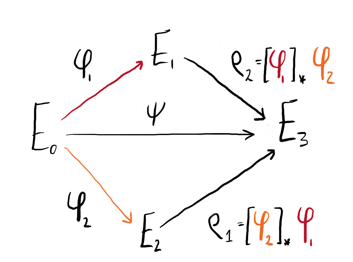
Figure 1: We can configure our isogenies and their pushforwards into a commutative diagram.
Via composition, the isogeny $\psi : E_0 \to E_3$ can be represented in two ways:
$$ \psi = [\phi_1]_\star \phi_2 \circ \phi_1 = [\phi_2]_\star \phi_1 \circ \phi_2 $$
Note on SIDH: For those who are familiar with SIDH, this is the SIDH square. When Alice and Bob send (the now notorious) auxiliary torsion points, they are sending the pushforward of the torsion basis under the action of their secret isogeny. This is what allowed for the construction of the shared secret $j(E_3) = j(E_3’)$.
Computing pushforwards in SageMath
Computing the pushforward of isogenies in SageMath is easy. Below we show a snippet that implements the above discussion.
# Assume that this data is already known
from known_data import E0, ϕ1_ker, ϕ2_ker

# Given isogenies and curves
ϕ1 = E0.isogeny(ϕ1_ker, algorithm="factored")
E1 = ϕ1.codomain()

ϕ2 = E0.isogeny(ϕ2_ker, algorithm="factored")
E2 = ϕ2.codomain()

# Compute the pushforward of the kernels
ρ1_ker = ϕ2(ϕ1_ker) # This will be a point on E2
ρ2_ker = ϕ1(ϕ2_ker) # This will be a point on E1

# Compute the isogenies to E3 and E3'
ρ1 = E2.isogeny(ρ1_ker, algorithm="factored")
ρ2 = E1.isogeny(ρ2_ker, algorithm="factored")

# The codomains of these isogenies are isomorphic
assert ρ1.codomain().is_isomorphic(ρ2.codomain())

# We can write the isogeny as
ψ = ρ1 * ϕ2 # E0 → E2 → E3
ψ_prime = ρ2 * ϕ1 # E0 → E1 → E3'
assert ψ.codomain().is_isomorphic(ψ_prime.codomain())
Pullbacks of isogenies
There is a mapping dual to the pushforward called the pullback. Given the same data as above, where the isogenies $\phi_1 : E_0 \to E_1$ and $\rho_2 : E_1 \to E_3$ are of coprime degree, the pullback of $\rho_2$ under the action of $\phi_1$ is denoted: $[\phi_1]^\star \rho_2 : E_0 \to E_2$.
Practically, we compute this by considering the image of $\ker(\rho_2)$ under the action of the dual isogeny $\widehat{\phi}_1$:
$$ \phi_j = [\phi_i]^\star \rho_j = [\widehat{\phi}_i]_\star \rho_j : E \to E / \langle \widehat{\phi}_i(\ker(\rho_j)) \rangle $$
Note that by using the pushforward and pullback maps, the entire SIDH square
can be recovered given any two coprime degree isogenies. We will use both of these mappings
in IdealToIsogenyFromKLPT() to compute various unknown isogenies from
isogenies that we can efficiently compute.
Computing pullbacks in SageMath
Below, we show a snippet that computes the above discussion of pullback isogenies.
# Assume that this data is already known
from known_data import E0, E2, ϕ1_ker, ρ2_ker

# Given isogenies and curves
ϕ1 = E0.isogeny(ϕ1_ker, algorithm="factored")
E1 = ϕ1.codomain()

ρ2 = E1.isogeny(ρ2_ker, algorithm="factored")
E3 = ϕ2.codomain()

# First, we need the dual of ϕ1
ϕ1_dual = ϕ1.dual() # This can be slow for large degree ϕ1

# Now we compute the image of ρ2_ker through ϕ1_dual
ϕ2_ker = ϕ1_dual(ρ2_ker) # This is a point on E0

# Compute the pullback isogeny
ϕ2 = E0.isogeny(ϕ2_ker, algorithm="factored")

# The codomains of these isogenies are isomorphic
assert ϕ2.codomain().is_isomorphic(E2)
Pushforwards and pullbacks of ideals
Via the Deuring correspondence, we can view an integral, cyclic ideal $I$ of norm $n(I) = N$ with left order $\OO_L$ and right order $\OO_R$ as equivalent to a cyclic isogeny $\phi : E \to E^\prime$ of degree $N$, for which $\End(E) \cong \OO_L$ and $\End(E^\prime) \cong \OO_R$.
We view the pushforward of an ideal $[I]_\star J$ as being the ideal $I_{[\phi_I]_\star \phi_J}$ equivalent to the isogeny $[\phi_I]_\star \phi_J$. Similarly, the pullback of the ideal $[I]^\star J$ corresponds to the isogeny $[\phi_I]^\star \phi_J = [\widehat{\phi}_I]_\star \phi_J$.
For isogenies, pushforwards and pullbacks take a kernel generator for some isogeny and map it to a new curve to produce an isogeny with the same degree but new (co)domain, the pushforward and pullback of an ideal is morally the same.
Let us align notation with the previous discussion of isogenies. We denote $I_1$ and $I_2$ to be ideals corresponding to $I_{\phi_1}$ and $I_{\phi_2}$, and $J_i = [I_j]_\star I_i$ to correspond to the pushforwards.
Explicitly, the pushforward $[I_2]_\star I_1$ takes the ideal $I_1$ with left order $\OO_0$ and right order $\OO_1$ and computes an ideal with left order $\OO_2$ and right order $\OO_3$. Similarly, the pullback $[I_1]^\star J_2$ takes the ideal $J_2$ with left order $\OO_1$ and right order $\OO_3$ and computes the ideal (equivalent to) $I_2$, with left order $\OO_0$ and right order $\OO_2$.
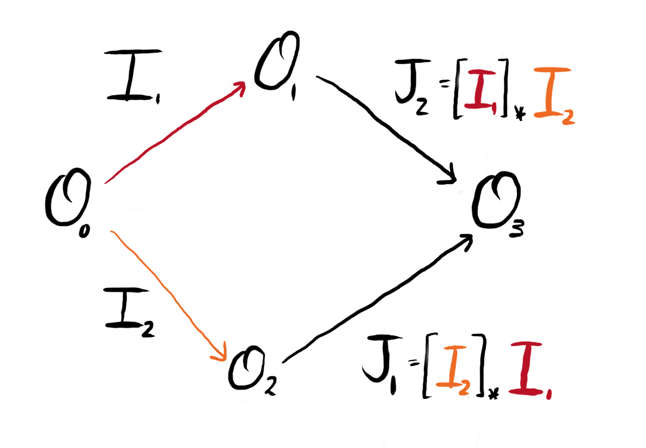
Figure 2: We can redraw Figure 1, replacing the isogenies with the equivalent ideals via the Deuring correspondence.
In SQISign, we will use these maps when we have an ideal $I$ with left-order $\OO$, and connecting ideal $I_\tau$ with left-order $\OO_0$ and right order $\OO$. Many of our algorithms are only efficient when the left order of the input ideal is the special extremal maximal order $\OO_0$, so when we wish to perform a computation with $I$, we first perform a pullback to find $K = [I_\tau]^\star I$, which has left-order $\OO_0$. We can then perform various computations on $K$ to obtain $K’$. Finally, we compute the pushforward $[I_\tau]_\star K^\prime$ and return something equivalent to $I$ with left order $\OO$.
Ideal computations
We do not need to perform the pushforwards and pullbacks at the level of isogenies, we can work directly with the ideals themselves. Let us review a few tricks which are outlined in Lemma 3 of the SQISign paper.
Let $I_i$ and $J_i$ be given as above, and let $K$ be the ideal corresponding to the isogeny $\psi : E_0 \to E_3$. We can compute the ideal $K$ connecting $\OO_0$ to $\OO_3$ from the multiplication of two ideals, or equivalently, from an intersection: $$ K = I_1\cdot J_2 = I_2\cdot J_1 = I_1 \cap I_2. $$ From the above, we see that the pushforwards can be recovered by multiplying with the inverse ideal: $$ J_i = I_j^{-1}\cdot (I_i \cap I_j) = I_j^{-1} \cdot K. $$ Finally, the pullbacks $I_i$ can be recovered by noticing that $[I_i]^\star J_j = [I_i]^\star [I_i]_\star I_j$ and taking the part of norm $N_i$ from the ideal of norm $n(I_2 J_1) = N_1 N_2$ in the following way: $$ I_i = [I_j]^\star J_i = I_j \cdot J_i + N_i \OO_0. $$
Computing pushforwards and pullbacks in SageMath
Below, we give the pushforward and pullback implementations
following the equations given above. SageMath has many functions which makes this fairly straightforward.
We note that ideal_generator() is the
function which given an left-$\OO$ ideal $I$ with $n(I) = N$,
finds $\alpha \in \BB$ such that $I = \langle \alpha, N \rangle = \OO \alpha + \OO N$.
def pushforward_ideal(O0, O1, I, Iτ):
    """
    Input: Ideal I left order O0
           Connecting ideal Iτ with left order O0
           and right order O1
    Output The ideal given by the pushforward [Iτ]_* I
    """
    assert I.left_order() == O0
    assert Iτ.left_order() == O0
    assert Iτ.right_order() == O1

    N = ZZ(I.norm())
    Nτ = ZZ(Iτ.norm())

    K = I.intersection(O1 * Nτ)
    return invert_ideal(Iτ) * K


def pullback_ideal(O0, O1, I, Iτ):
    """
    Input: Ideal I with left order O1
           Connecting ideal Iτ with left order O0
           and right order O1
    Output The ideal given by the pullback [Iτ]^* I
    """
    assert I.left_order() == O1
    assert Iτ.left_order() == O0
    assert Iτ.right_order() == O1

    N = ZZ(I.norm())
    Nτ = ZZ(Iτ.norm())

    α = ideal_generator(I)
    return O0 * N + O0 * α * Nτ
SQISign response
Let us end this discussion with an efficient computation of a product of ideals
needed when computing the response() for SQISign.
In SQISign’s response, we are asked to find the value of $\bar{I}_\tau \cdot I_\psi \cdot I_\phi$ with $\psi : E_0 \to E_1$, $\phi : E_1 \to E_2$ and $\tau : E_0 \to E_A$, such that the product of ideals corresponds to the isogeny $\sigma : E_A \to E_2$.
Using the above notation, we have $I_\phi = J_2$ and $I_\psi = I_1$. So, we can use the identity: $$ J_2 = I_1^{-1} \cdot (I_1 \cap I_2) \Rightarrow I_1 \cdot J_2 = (I_1 \cap I_2). $$
As a result, $I_\psi \cdot I_\phi$ can be computed directly from the intersection of $I_\psi$ and the pullback $[I_\psi]^\star I_\phi$ (which would be $I_1$ in the above notation). This means we can save computing $I_\phi$ itself (which is slow as its left order is not $\OO_0$) and instead work with the pullback which does have left order $\OO_0$ and so allows for efficient computations.
Below we include a snippet which shows this computation as it appears in SQISign.py.
from isogenies_and_ideals import kernel_to_ideal
from known_data import E0, Iτ, ϕ_ker, ψ_ker

# Given isogenies and curves
ψ = E0.isogeny(ψ_ker, algorithm="factored")
E1 = ψ.codomain()

ϕ = E1.isogeny(ϕ_ker, algorithm="factored")
E2 = ϕ1.codomain()

# First, we need the dual of ψ
ψ_dual = ψ.dual() # This can be slow for large degree ϕ1

# Now we compute the image of ϕ_ker through ψ_dual
ϕ_ker_pullback = ψ_dual(ϕ_ker) # This is a point on E0

# Compute the ideal Iψ from ψ_ker
Iψ = kernel_to_ideal(ψ_ker, ψ_ker.order())

# Compute the pullback isogeny
Iϕ_pullback = kernel_to_ideal(ϕ_ker_pullback, ϕ_ker_pullback.order())

# Compute the product Iψ * Iϕ
IψIϕ = Iψ.intersection(Iϕ_pullback)
assert IψIϕ.norm() == Iψ.norm() * Iϕ_pullback.norm()

# Compute the final product of ideals
# I = Iτ_bar * Iψ * Iϕ
Iτ_bar = Iτ.conjugate()
I = Iτ_bar * IψIϕ
assert I.norm() == Iτ_bar.norm() * IψIϕ.norm()